How to Alphabetize in Google Sheets: 4 Easy Methods

To alphabetize data in Google Sheets, use a SORT formula when you want a live, separate sorted result, or use the built-in sort commands when you want to rearrange existing rows. The four methods below cover a single list, complete multi-column records, an entire worksheet, and a selected range with advanced rules.

1. Use SORT to alphabetize one column

The SORT function returns an alphabetized copy of a range, leaving the source list in place. This is useful for customer names, product names, or any list that may change over time.

1. Put your original values in a column, with a header in row 1 if needed.
2. Select an empty cell where the sorted results can expand. Make sure the cells below it are empty.
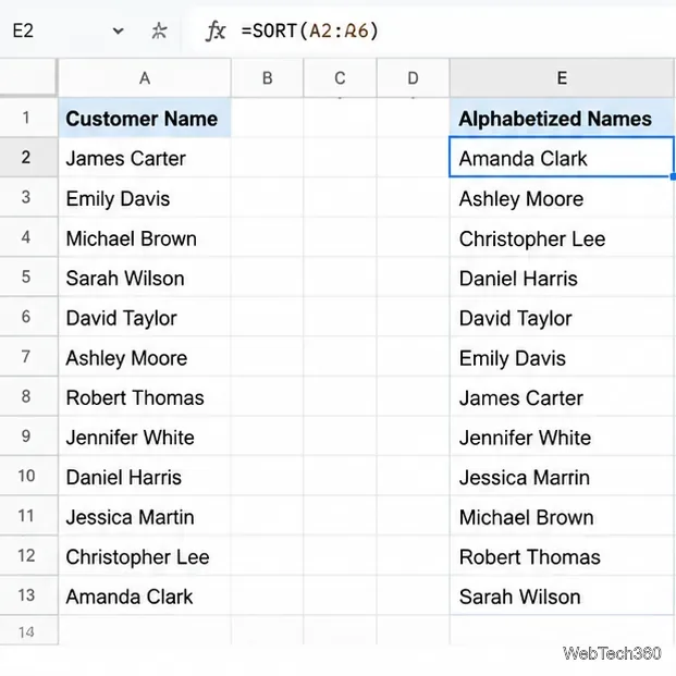
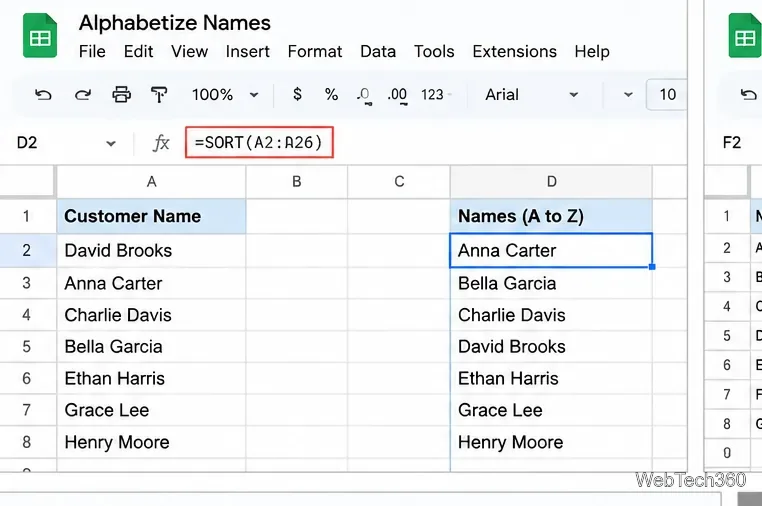
3. Enter =SORT(A2:A26) and press Enter. Replace the example range with your actual data range.

By default, SORT uses ascending order, so text appears from A to Z. To sort Z to A, use =SORT(A2:A26,1,FALSE). The formula output updates as source values change, provided its destination range remains clear. If you see a #REF! error, check for existing values blocking the result.

2. Use SORT to keep multiple columns together

When names, email addresses, states, and statuses belong to the same record, sort the entire row range—not just one column. Sorting a single column by itself can mismatch names with their details.

1. Choose a blank area or a separate sheet for the sorted output.
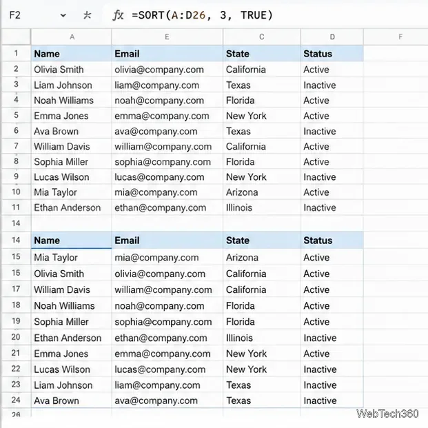
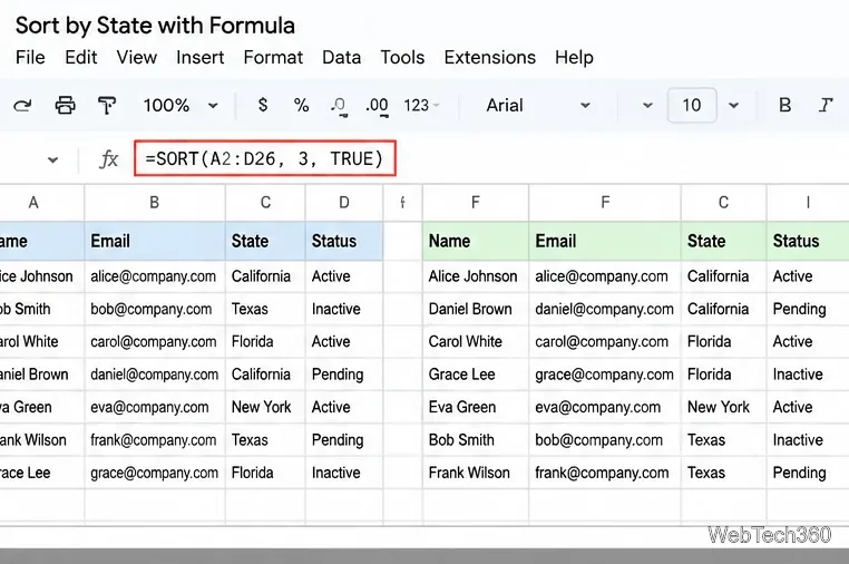
2. Enter a formula such as =SORT(A2:D26,3,TRUE).
3. Press Enter. The range A2:D26 is returned in ascending order based on its third column, C. In this example, column C contains State.

The second argument is the sort-column index relative to the range: 1 means the first column in the selected range, 2 the second, and so on. TRUE means ascending; FALSE means descending. You can add further sort-column and order pairs to break ties, for example =SORT(A2:D26,3,TRUE,1,TRUE) sorts by State first, then by the first column.

3. Sort the entire sheet with the column menu

Use this option when you want to rearrange the original worksheet instead of creating a separate formula result. It sorts the sheet based on one column and keeps each row's values together.

1. If the first row contains headings, choose View → Freeze → 1 row so the header stays visible.
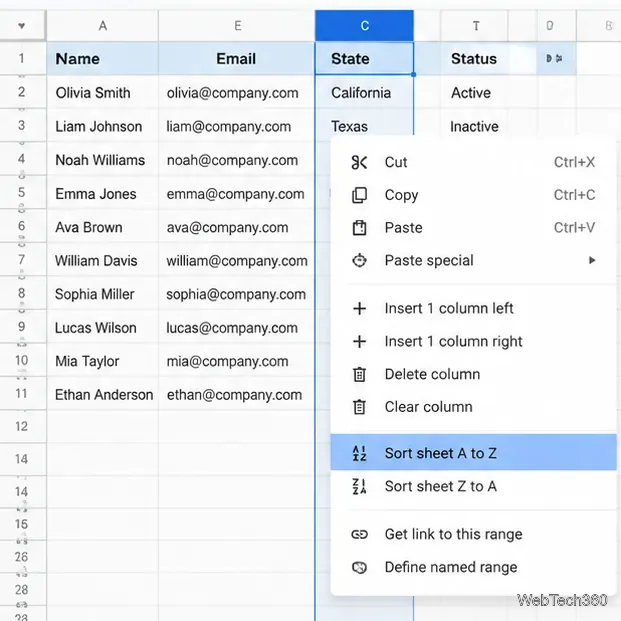
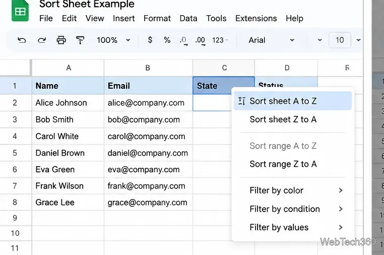
2. Right-click the letter at the top of the column you want to sort by.
3. Choose Sort sheet A to Z or Sort sheet Z to A.

Before sorting, confirm that the worksheet's related data is arranged in consistent rows and that there are no unrelated tables elsewhere on the same sheet. A sheet-level sort is intended to rearrange sheet data, so make a copy first if you are unsure how it will affect the layout.

4. Use Advanced range sorting options

Advanced range sorting is the best choice when you need to sort a specific table, identify its header row, or apply multiple levels such as State first and Name second.

1. Select the full table range, including every column that should stay together.
2. Open Data → Sort range → Advanced range sorting options.
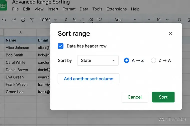
3. Check Data has header row if the selected range includes column headings.
4. Choose the primary sort column and select A → Z or Z → A.
5. To add a tie-breaker, click Add another sort column, choose the next column and order, then click Sort.

For example, sort by State A to Z, then add Name A to Z to alphabetize customers within each state. Unlike the formula method, this command rearranges the selected source range. Selecting the full table is important so each record stays intact.

Which method should you choose?

• One column, live result: use =SORT(A2:A26).
• Full records, live result: use SORT with the full range and sort-column index.
• Quickly rearrange the whole sheet: use the column menu's Sort sheet command.
• Sort one table with headers or tie-breakers: use Advanced range sorting options.

Common alphabetizing problems

• The header gets mixed into the list: exclude the header from a formula range, or enable Data has header row in the range dialog.
• Details no longer match the names: select the complete table or use a formula that returns all related columns.
• The formula cannot expand: clear cells in the output area or move the formula to a blank range.
• The order looks unexpected: check for leading spaces, inconsistent spelling, blank cells, or values stored in different formats.

For exact menu names and formula syntax, consult Google's official guide to sorting and filtering data in Google Sheets and the SORT function reference.