How to Subtract in Google Sheets: A Practical Full Guide

To subtract in Google Sheets, enter a formula such as =A2-B2 in a blank cell and press Enter. Start with an equals sign, then use the minus operator. To calculate more rows, fill the first formula down the column.

Subtract two cells with a formula

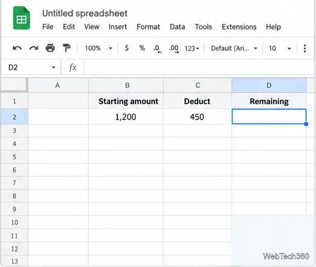
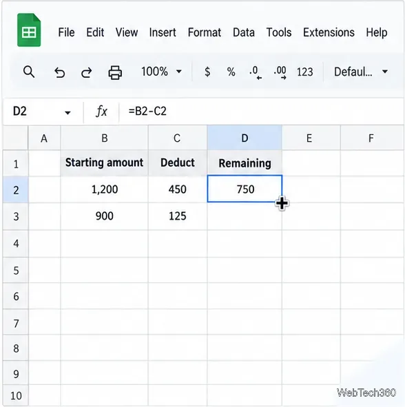
For this example, column B holds a starting amount, column C holds the deduction, and column D shows what remains. In row 2, B2 is 1,200 and C2 is 450, so the result should be 750.

1. Enter numeric values in the two input columns. Add headers if they will help you identify each value.
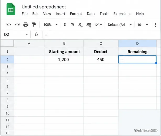
2. Select the result cell in the same row, such as D2, and type =. Every formula starts with an equals sign.

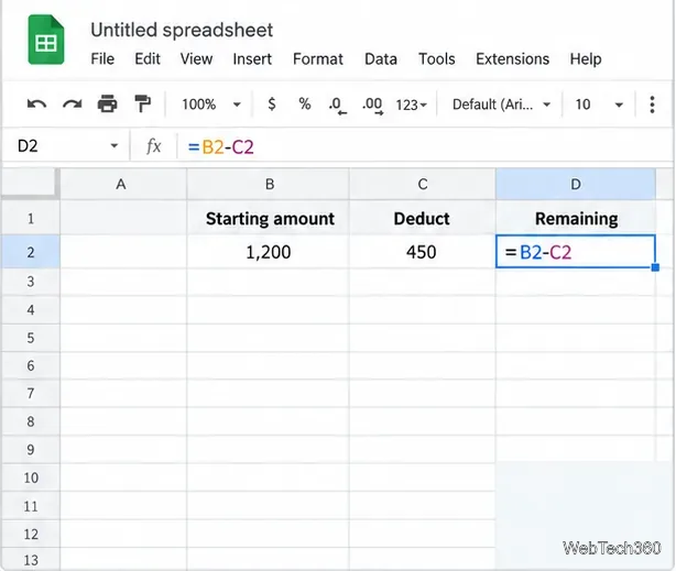
3. Type or select the first cell reference, type a minus sign (-), then type or select the second reference. The complete formula is =B2-C2. You can click cells while editing to insert their references.
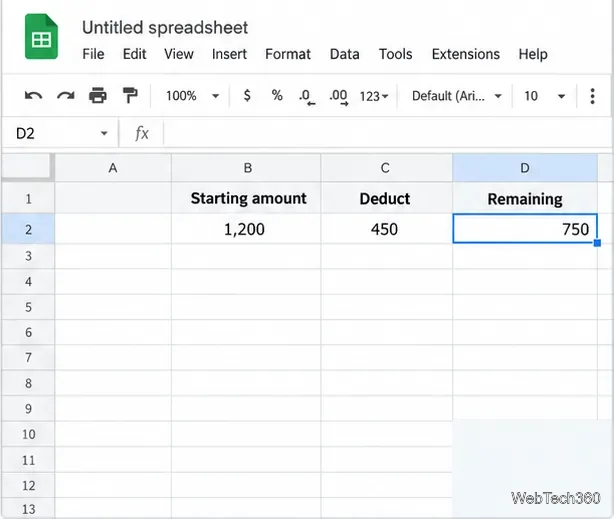
4. Press Enter. Sheets calculates the answer in D2 and recalculates it when B2 or C2 changes.

Subtraction follows the order you write: =B2-C2 means B2 minus C2. A negative result is valid when the second value is larger. For money, keep cells numeric and apply a currency number format instead of adding a symbol to the formula. See Google’s guide to formulas and functions for more on entering and editing formulas.

Subtract multiple values

For a quick calculation without cell references, enter =25-7. To subtract several values from one starting amount, use =B2-C2-E2. If the deductions are in a range, subtract their total with =B2-SUM(C2:E2).

Sheets also supports =MINUS(B2,C2). This function returns the first value minus the second and takes exactly two arguments. The minus operator is shorter for most everyday formulas. Google’s MINUS function reference lists its syntax.

Apply the formula to more rows

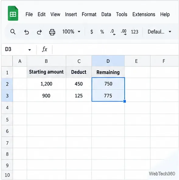
After entering =B2-C2 in D2, select the cell and drag the small fill handle at its lower-right corner through the rows that need results.

When copied down, relative references adjust: the next formula becomes =B3-C3. With B3 at 900 and C3 at 125, D3 displays 775. Check a copied cell if you want to confirm its row numbers.

For a keyboard method, select the range from the completed formula through the last destination cell, then use Fill down: Ctrl+D on Windows or ChromeOS, or ⌘+D on Mac. Google lists these on its Sheets keyboard shortcuts page.

Keep one cell reference fixed

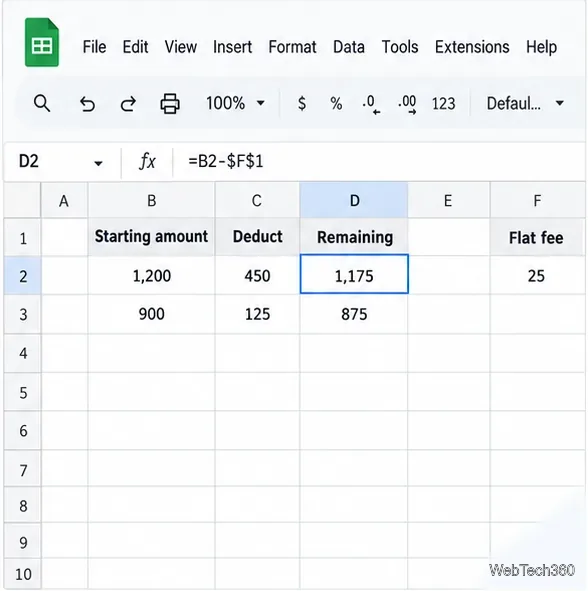
To subtract the same fee from every row, put it in F1 and enter =B2-$F$1 in D2. Fill the formula down: B2 changes to B3, while $F$1 stays fixed. Dollar signs lock both the column and row; $F1 locks only the column, and F$1 locks only the row.

View or edit a formula

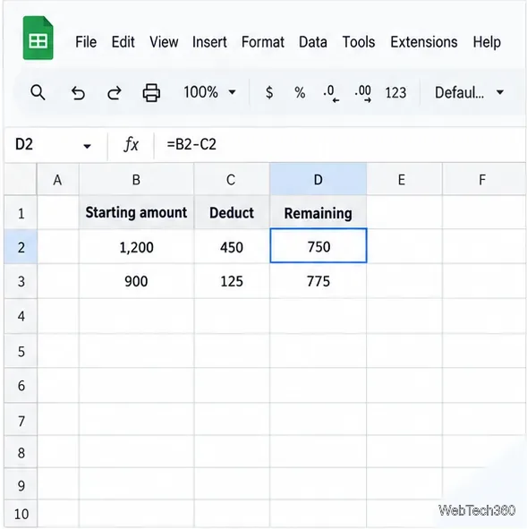
Click a result cell to see its formula in the bar beside the fx indicator. Double-click the cell or edit the formula bar to make a change, then press Enter.

To show formulas across the grid instead of results, press Ctrl+~ on Windows or ChromeOS, or ⌘+~ on Mac. Press the shortcut again to return to results. Use this toggle to review many formulas at once.

Fix common subtraction problems

• The cell displays the formula: turn off formula display, remove any leading apostrophe, and check that the cell is not formatted as plain text. Change it to Automatic and re-enter the formula.
• You see #VALUE!: confirm that the referenced cells contain numbers, not labels or text imported from another source.
• Filled results look wrong: inspect a formula in the formula bar and confirm its row references point to the intended inputs. Lock references that must stay fixed with dollar signs.
• The result is negative: the subtracted amount is larger than the starting value. Reverse the references only if you want the opposite difference.

The basic pattern is =first value-second value. Use fill down for repeated rows and an absolute reference when a shared input must stay in place.