How to Move a Picture in Microsoft Word
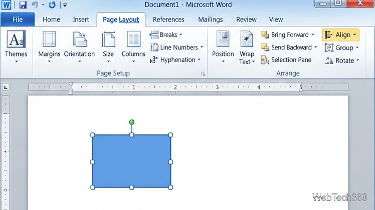
Learn how to drag a picture in Word, choose text wrapping, keep it with a paragraph or fix it on the page, and troubleshoot images that will not move.
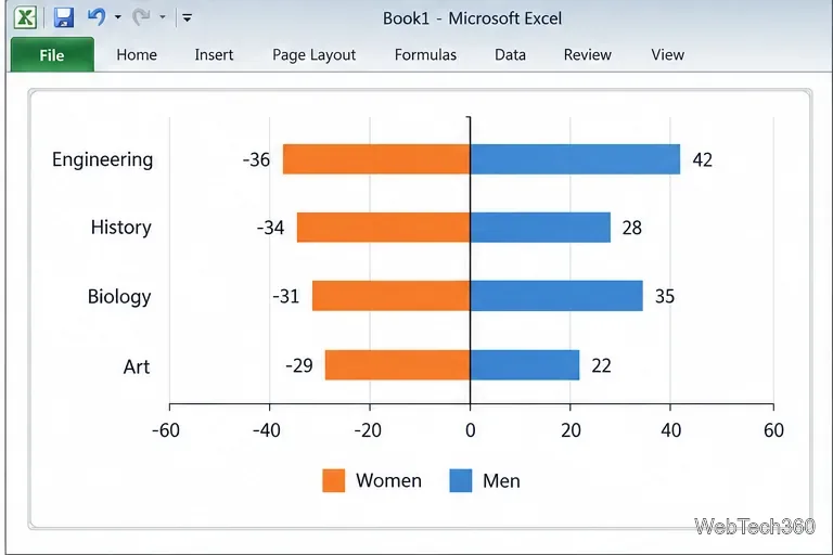
A comparative histogram in Excel 2010 is usually a mirrored horizontal bar chart: one group extends left from zero and the other extends right. It compares two values across the same categories, such as student counts by department. The negative numbers are a plotting device, not negative counts.
This chart is not a statistical histogram. A true histogram groups numeric measurements into bins and shows how often values fall in each bin. Microsoft documents histograms and bar charts as separate chart types; use this mirrored method when you want to compare two groups category by category.
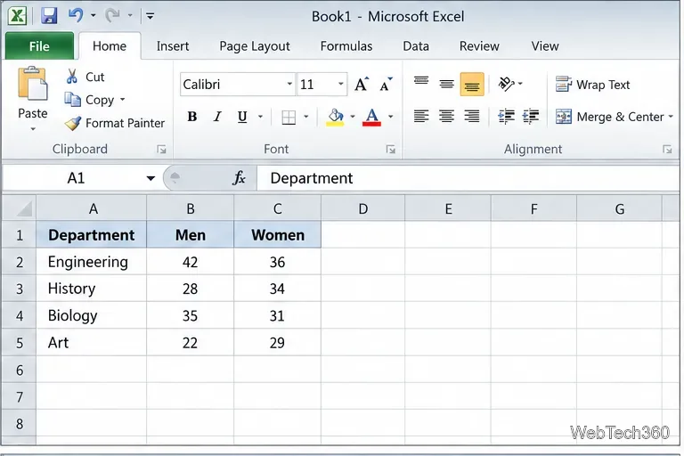
Keep one row per category and put each group in its own column. For example:
| Department | Men | Women |
|---|---|---|
| Engineering | 42 | 36 |
| History | 28 | 34 |
| Biology | 35 | 31 |
| Art | 22 | 29 |
Do not replace your original counts with negative values. Make a separate, adjacent chart-ready block and use formulas so the source table stays intact.
Use clear column headings and numeric values, with no blank rows inside the range. Each row should represent the same department for both groups. Each row must use the same category for both groups.
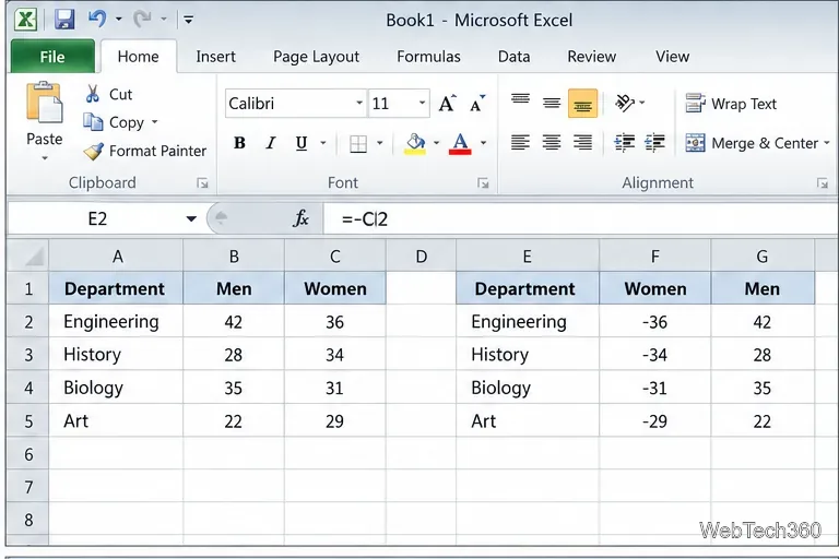
In an empty area, create three adjacent columns headed Department, Women (left), and Men. If the source columns are A:C, enter =A2 in the helper department cell, =-C2 for Women, and =B2 for Men. Fill the formulas down for each department. The minus sign makes the women’s bars extend left; the original counts remain positive in the source table.
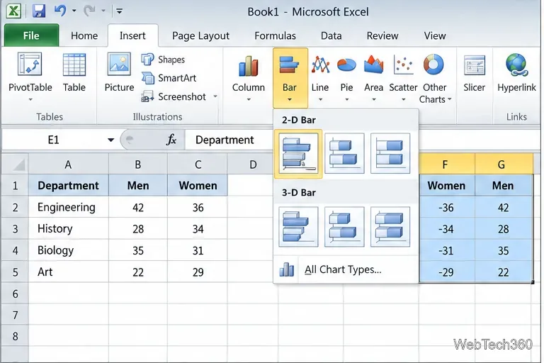
Select the full chart-ready range, including the headings. On the Insert tab, open Bar in the Charts group and choose 2-D Clustered Bar. In Excel 2010, the command appears on the classic Ribbon; the exact button layout can vary with window size. Avoid stacked or 3-D bars because this comparison needs two series to share each category row.
Check that department names appear as the vertical category labels, Women extends left of zero, and Men extends right. The initial value axis will show negative numbers on the left; that is expected. If Excel plotted the wrong fields, right-click the chart and choose Select Data to check the category-label range and each series. If both groups extend the same way, check the helper formula and the selected range.
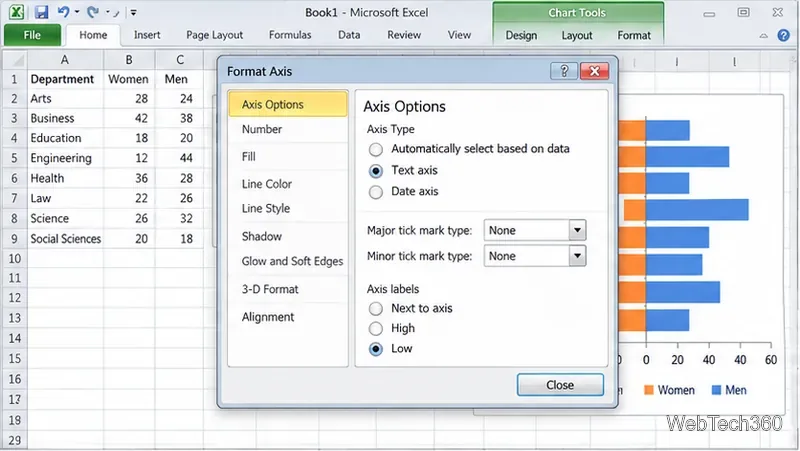
Right-click a department label and choose Format Axis. Under Axis Options, set Major tick mark type and Minor tick mark type to None, then set Axis labels to Low. This places the category names at the left edge of the plot and removes small ticks that add clutter. If the first department appears at the bottom, use Categories in reverse order in the same dialog to choose the order you prefer.
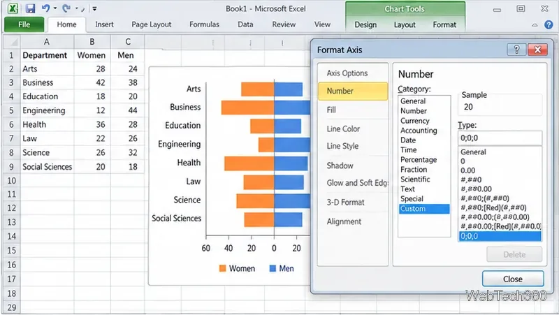
Right-click the horizontal number axis and choose Format Axis. In Axis Options, give the axis symmetric minimum and maximum bounds based on the largest count. For a largest value of 42, for example, use -50 and 50 so both sides have the same scale. Then open Number, choose Custom, and enter 0;0;0 as the format code. In this three-section format, positive values, negative values, and zero each display without a minus sign on the axis. Click Add if Excel 2010 shows that button, then close the dialog. Number formatting changes the labels, not the helper values used to draw the bars.
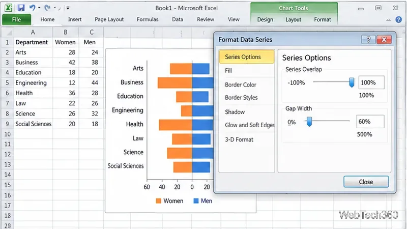
Right-click a bar and choose Format Data Series. Under Series Options, set Series Overlap to 100% so each department’s two bars line up around the same row. Set Gap Width to about 60% to start; lower values make thicker bars, while higher values leave more space between departments. Adjust it to fit.
Keep the legend and name the series Women and Men. On Chart Tools > Layout, add a title such as Students by Department. Because the number axis now shows positive-looking values on both sides, add a small text box below the plot that says Women ← | → Men, or otherwise label which group is on each side. In Excel 2010, choose Text Box on the Layout tab. Leave data labels off unless you also format negative labels; the axis number format does not change labels attached directly to bars.
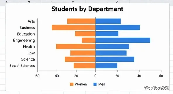
This chart compares counts. If group sizes differ and you need rates or proportions, calculate those percentages first. Microsoft’s current chart guidance sometimes uses newer pane names, but the same chart and axis controls apply to Excel 2010’s classic dialogs.
Learn how to drag a picture in Word, choose text wrapping, keep it with a paragraph or fix it on the page, and troubleshoot images that will not move.
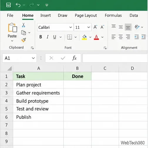
Learn how to insert a checkbox in Excel with the in-cell tool, count checked items with formulas, or add a linked Form Control in older desktop versions.
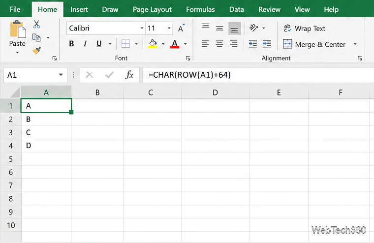
Generate A to Z, lowercase letters, or labels beyond Z in Excel with a fill-handle formula, SEQUENCE, or a reusable custom list.
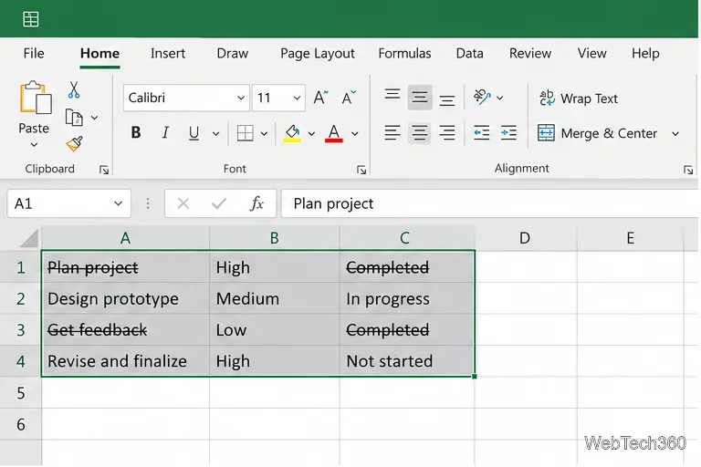
Learn how to strikethrough in Excel on Windows, Mac, and the web, format part of a cell, and remove the line without deleting its value.
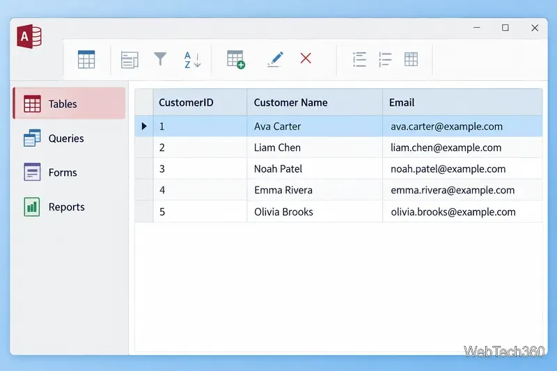
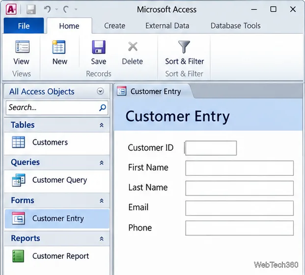
Microsoft Access is a Windows database app for storing related records, building queries, creating data-entry forms, and generating reports. Learn how it works and when it fits.
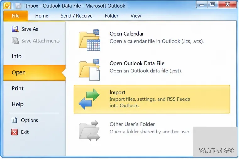
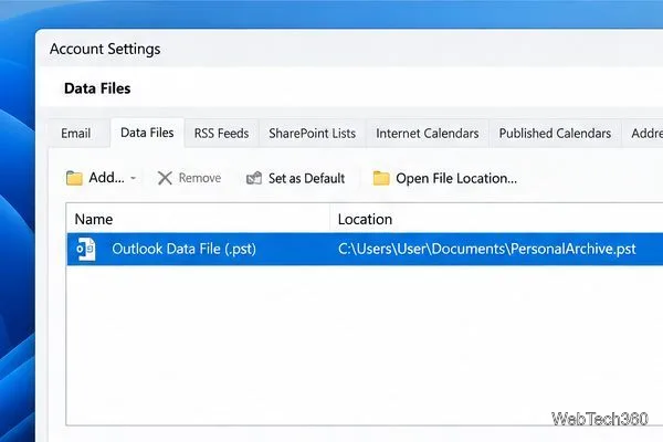
Learn how to import a PST into Outlook 2010 or export mail, contacts, calendar, and tasks. Follow the correct menus and avoid missing folders or duplicates.
Learn how to adjust gridline height and width in Word 2010, change visible line frequency, and set the underlying horizontal and vertical drawing-grid spacing.
Recover a forgotten Outlook PST password with Kernel’s current steps, including how to identify the right file, make a backup, and check the tool’s limits.
Use the LiveWeb add-in to place a website on a PowerPoint slide, set its size and refresh behavior, and check compatibility before presenting.
Set an Access 2010 database application to open directly to a data-entry form, hide object lists, limit menus, and check the setup before sharing.